


In our previous article, we completed our look at mechanical properties by discussing how allowable stresses are determined. In this article we are going to look at the last pieces of information we need to conduct a pipe stress analysis, i.e. stress intensification factors and flexibility factors.
When engineers conduct a pipe stress analysis, they construct a mathematical model of the piping system. The basic elements of the model are beam elements because, as far as loads other than pressure are concerned, a piping system is essentially a combination of connected beams. That’s fortunate because the equations for stresses in a beam are simple and exact; no approximations are required. Unfortunately, only pipe itself behaves as a beam element. The other components in a piping system, i.e. the fittings such as elbows, tees, reducers, etc., display more complex stress behaviors compared to the pipe.
So in order to correctly predict the stresses in the fittings, we need to apply “fudge factors” to the stresses calculated for pipe. These fudge factors are called stress intensification factors or “SIFs”. For FRP fittings, SIFs are defined as the ratio of the maximum stress in the fitting to the maximum stress in a pipe when exposed to the same loading. For example, let’s assume that a section of pipe is exposed to a bending moment equal to M. This could be the bending moment due to the weight of the pipe and contents midspan between two supports. The maximum bending stress in the pipe is simple to calculate and is equal to:

where:
Sb = Bending stress
M = Bending moment
Z = Section modulus of the pipe. This is a geometrical property of the pipe dependent only on the diameter and thickness of the pipe.
Now, if there were a fitting such as an elbow or a tee at the midspan between the supports and therefore exposed to the same bending moment, the maximum stress in the fitting would likely be different (and probably higher) than in the pipe. The Finite Element Analysis (FEA) image below, of a reducing tee, illustrates how the local stresses in a fitting can be much higher than in the adjacent pipe.
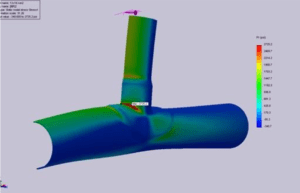
To predict the maximum stress in a fitting, we apply an SIF to the equation above, i.e.

where:
i = Stress intensification factor (SIF)
Where do the values for SIFs come from? If we were analyzing metallic piping systems, we could find SIFs for a wide range of fittings in the ASME piping codes, i.e. B31.1 and B31.3. But these values typically do not apply to FRP fittings due to differences in geometries and differences in definitions of SIFs between FRP and metallic fittings. ASME NM.2 contains expressions for calculating SIF’s for a limited number of fittings and laminate constructions, but to obtain appropriate SIF’s for FRP fittings in general, it is often necessary to generate values by testing or by using FEA such as that illustrated in the image above. In some cases, FRP piping manufacturers have utilized empirical values that have proven to be conservative over many years, and these too can be helpful. In any case, the FRP piping manufacturer should be consulted for appropriate SIF’s for their fittings.
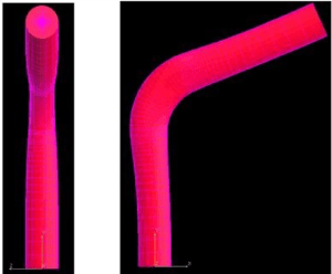
A second factor that should be considered in a pipe stress analysis is the flexibility factor, or “k”. This factor is used to predict how much greater the rotational deformation of a fitting will be compared to that of an equivalent length of pipe. The k factor for many fittings such as tees and reducers is simply taken to be 1.0 as the deformation of the fittings is essentially the same as the pipe. The same is not generally true of elbows. When a bending moment is applied to an elbow, the elbow will ovalize as illustrated in these FEA images.
This ovalization results in the rotation of one end of the elbow relative to the other being different than would be the case for pipe, and in fact, is typically several times that of the pipe. This is an important characteristic when the piping system is being analyzed for displacement loadings such as temperature differential. The presence of an elbow in a section of piping can provide a significant amount of flexibility in the piping run, thereby keeping the thermal loads and hence stresses, to manageable levels.
Where do we find values for k? Again, if we were analyzing metallic piping systems, we could find k’s in the ASME piping codes, i.e. B31.1 and B31.3. But these values are typically not appropriate for FRP fittings due to differences in geometries, constructions, and properties of FRP fittings compared to metallic fittings. So as with SIF’s, we need to utilize testing or FE analysis to determine k values. FRP piping manufacturers should be consulted for appropriate k’s for their fittings.
In our next article, we will take one last look at pipe system design by discussing how all the information from the last several articles comes together in a pipe stress analysis.
Previous article in the series: Strength Properties
Next in the series: How Pipe Stress Analysis is Carried Out